Lecture 9: Self-Organising Maps

$K$-means Clustering

This is an iterative algorithm for grouping data into distinct sets.

Algorithm

1. Estimate the initial centroid values $c_1^0, \ldots , c_K^0$
2. Set $i=0$
3. $\forall n \in 1...N , \forall k \in 1...K,$ calculate $d(x_n,c_k^i)$
4. $\forall k \in 1...K$:
   1. Let $X^i(k)$ be the set of $x_ns$ that are closest to $c_k^i$
   2. Define $c_k^{i+1}$ to be the average of the data points in $X^i(k)$
      $c_k^{i+1} = \frac{1}{|x^i(k)|} \sum_{x\in X^i(k)}x$
   3. i++, return to step 3

See slides for examples

Optimality

We can now ask the question: is the set of $k$ centroids, $\hat{C}$ created via $k$-means globally optimal? I.e. does the following hold?

$D(C,X) \geq D(\hat{C},X)$

No! $k$-means is only guaranteed to find a local optimum with it's final result being dependent on the initial centroid guesses

Alternative to $K$-means

In $k$-means we calculate the distances between all data points and all centroids before any update takes place. Instead, we can update centroid locations based on seeing a single data point $x_n$

'Online' Clustering

Online clustering updates centroids with each sample using the following equation:

$c_k^{\text{new}} = c_k^{\text{old}} + \eta(x_n - c_k^{\text{old}})$

Where $\eta>0$ is the learning rate.

• If $\eta$ is too small convergence will be too slow
• If $\eta$ is too big, algorithm will be unstable

Our solution to this is to start with a big value of $\eta$ and to shrink it over time.

$\eta(t) = \eta(0) \times e^{\frac{-t}{\tau}}$

Where $\tau$ is the time scale, determining how fast $\eta$ will decrease.

This process is similar to that of annealing

Algorithm

1. Choose the number of centroids, $K$

2. Randomly choose an initial codebook $\{c_1,\ldots,c_K\}$

3. $\forall x_n \in X$:

   1. Find the closest centroid $c_{i(n)}$
   2. Move $c_{i(n)}$ closer to x_n
      $c_{i(n)}^{\text{new}} = c_{i(n)}^{\text{old}} + \eta(t)\left(x_n-c_{i(n)}^{\text{old}}\right)$

   where $\eta(t) >0$ is a small learning rate that reduces with time as determined by the equation:
   $\eta(t) = \eta(0) \times e^{\frac{-t}{\tau}}$
   where $\tau$ is the timescale

Enhancements to Online Clustering

• Batch Training: accumulates changes to centroids over small subsets of the training set
• Stochastic batch training: accumulates changes to centroids over small randomly chosen subsets of the training set

Neighbourhood Structure

Neighbourhood structuring is the process by which each point in the centroid set is connected it's nearest neighbours. The number of neighbours that it is directly connected to depends on the number of dimensions the structure is imposed for.

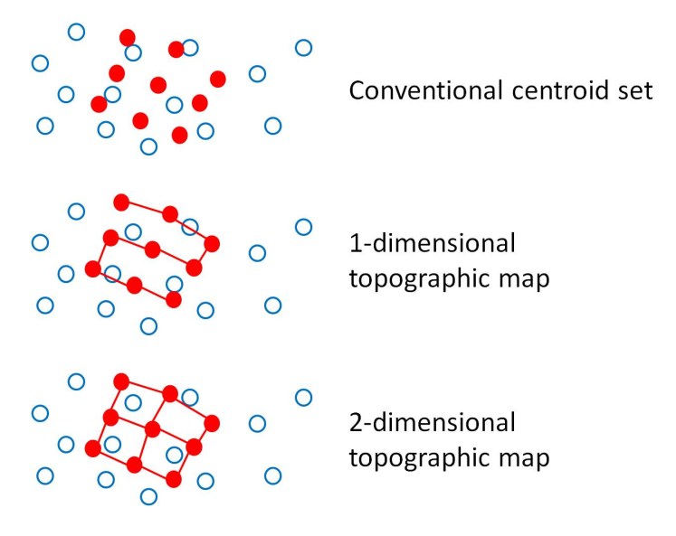
We can imagine the connections between these centroids in a neighbourhood as elastic bands whereby when we move one centroid closer to a data point to further reduce the distortion of the dataset we also move all other centroids by an amount proportional to how closely connected each centroid is to the one we just directly moved.

1 Dimensional Neighbourhood Structure

In 1 Dimension each centroid is directly connected to one other centroid, with ultimately each centroid being connected to all other centroids in the neighbourhood.

To define a neighbourhood structure you require a definition of distance between the members of the neighbourhood.

So for a neighbourhood centered on centroid $j$ with distance $d$ we can define the set of all other centroids where the indices of the centroids are less than or equal to $d$ as:

$N_j(d) = \{c_k \big\vert \;|k-j| \leq d \}$

An illustration of a 1D neighbourhood defined with a range of distances can be seen below

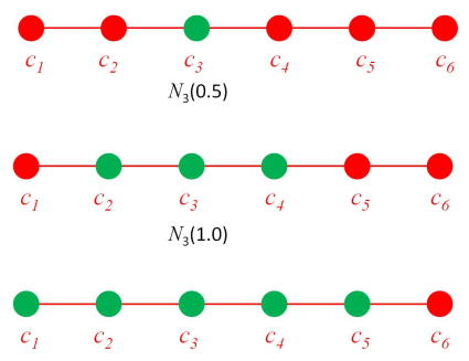
Note that these neighbourhoods are defined on the centroid index not the centroid coordinates!

2 Dimensional Neighbourhood Structure

Similarly we can define our neighbourhood structure in 2 dimensions with the equation:

$N_{ij}(d) = \left\{ c_{kl} \big\vert \lVert \begin{bmatrix} k \\ l \end{bmatrix} - \begin{bmatrix} i \\ j \end{bmatrix} \rVert \leq d \right\}$

Constrained Clustering

The aim of Constrained clustering using self-organising or topographic maps is to discover $N$ dimensional structure of high dimensional data by clustering whilst constraining our centroids to lie in a $N$ dimensional 'elastic'

Where the $N$ dimensions are the dimensionality of the neighbourhood structure.

Recalling our equation for Online Clustering

$c_{i(n)}^{\text{new}} = c_{i(n)}^{\text{old}} + \eta(t)\left(x_n-c_{i(n)}^{\text{old}}\right)$

We can now define our update rule for Constrained clustering using a topographic map as:

$c_k^{\text{new}} = c_k^{\text{old}} + h(i(n),k) \times \eta(t) \times (x_n - c_k^{\text{old}})$

Where $h(i(n),k)$ indicates how close the $k^{\text{th}}$ centroid is to the centroid $c_{i(n)}$ closest to $x_n$

What do we choose for $h(x,y)$ ?

Any candidate function must satisfy:

1. $h(i(n),i(n) =1$
2. $h(i(n),k)$ decreases as $c_k$ becomes further away from $c_{i(n)}$

One possible function is:

$h(i(n),k) = \exp\left[ \frac{-\|i(n) - k \|}{\sigma} \right]$

Where $\sigma$ is the neighbourhood width or strength of the elastic

In choosing a value for $\sigma$ we can employ Simulated Annealing whereby we initially choose a high value to allow for broad cooperation between centroids but gradually reduce the value as the algorithm runs.

One scaling factor could be:

$\sigma(t) = \sigma(0) \times \exp\left[ \frac{-t}{\nu}\right]$

where $\nu > 0$ is the timescale and $\sigma(0)$ is the initial neighbourhood weight