In Lecture 5 we derived the per-example cost function:
Ci=j=1∑m21(yj(i)−ajL)2(1)
where ajL is the output of the model
Using the maximum likelihood method under the assumption that the predicted output ajL has a Gaussian (normal) distribution. This assumption is acceptable for regression problems
However, when we look at classification problems with m discrete class labels {1,⋯m} it makes more sense to have one output unit Pj per class, j where Pj is the probability of the example falling into class j
These units therefore have to satisfy the following conditions:
- 1≥Pj≥0∀j∈{1⋯,m}
- ∑j=1mPj=1
Diagrammatically, we replace the last layer of our network with a "softmax" layer
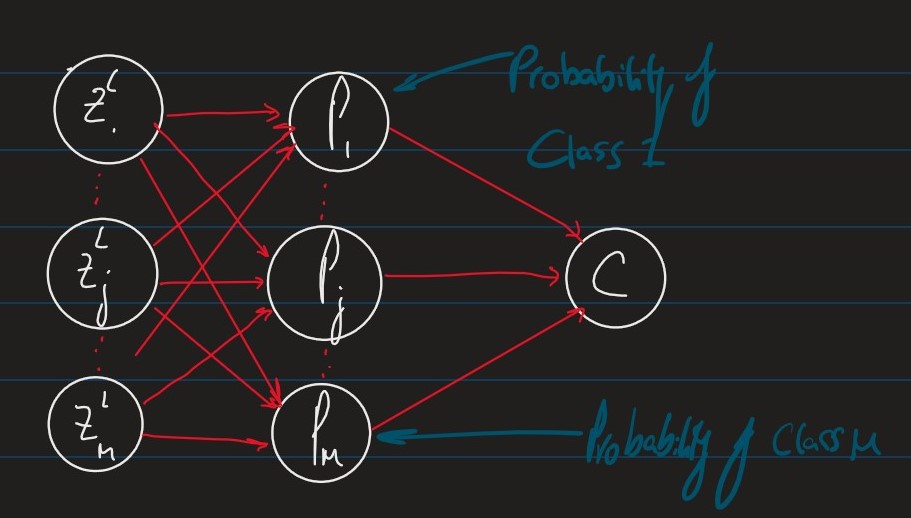
Pj=QezjL(2)
where:
Q=j=1∑mezjL(3)
Here we use the exponential function to make certain that our probability stays positive and that the total probability doesn't exceed 1, a quick proof of this is as follows:
j=1∑mPj=Q1j=1∑meziL=QQ=1(4)
Then, as we have bounded our probabilities, we can say:
Py=Pwb(y∣x)(5)
i.e the probability of class, y∈{1,⋯,m} given input x
Given n independent observations (x1,y1),⋯,(xn,yn) where yi∈{1,⋯,n} is the class corresponding to the input xi, the likelihood of weigth and bias parameters w,b is:
L(w,b∣(x1,y1),⋯,(xn,yn))=i=1∏nPwb(yi∣xi)=i=1∏nPyi(6)
We can define a cost function using the maximum likelihood principal.
C=−logL(w,b∣(x1,y1),⋯,(xn,yn))=n1i=1∑nCi(7)
where:
Ci=−logPwb(yi∣xi)=−logPyi=logQ−zyiL(8)
To apply gradient descent to minimise the cost function, we need to compute the gradients.
δwjklδC=i=1∑nδwjklδCi(9)
δbjlδC=i=1∑nδbjlδCi(10)
To compute these using backpropogation, we need to compute the local gradient for the softmax layer:
δjL:=δzjδCi(11)
δjL=δzjLδCi=Pj−δyij
where
δab={10if a=botherwise
- This is also known as the Kronecker-Delta function
δzjLδCi=−δzjδlogP(yi∣xi)=−δzjδlogPyi=−δzjδ(zyi−logQ)=−(δyij−δzjδlogQ)=−(δyij−Q1ezj)=Pj−δyij□(12)
Neural networks are usually implemented with fixed length representations of real numbers.
Obviously, these representations are finite representations of a uncountably infinite set R
For instance, the maximal value of the float64 data type in NumPy can represent is ≈1.8×10308
When computing the numerator in QezjL we can easily exceed this limit
For any constant,r:
Pj=∑kezkLezjL=er⋅∑kezkLer⋅ezjL=∑kezkL+rezjL+r(13)
To avoid too large exponents, it is common to implement the softmax function as the rightmost expansion above with the constant:
r:=−kmaxzkL(14)